
In our work towards practical Quantum 1-Shot Signatures, we have two main problems to solve:
- Building cryptographic gadgets called equivocal hash functions.
- Baking them into quantum circuits, and simplify the latter enough that the they can be run on quantum computers in the not-too-far future.
For the quantum side of our work, we rely heavily on modern diagrammatic techniques, using languages such as the ZX calculus and the ZH calculus to design, modify and optimise our quantum circuits. This post introduces the ZX calculus, the most widely adopted diagrammatic language for digital — that is, qubit-based — quantum computing
The ZX calculus is a diagrammatic language which can be used to design and reason about quantum circuits, originally devised by Coecke and Duncan. A cool observation about it is that the very same rewrite rules which are used to reason about quantum circuits can also be leveraged to simplify them, performing the same computation while optimising some cost function of interest. For example, ZX-based techniques are State-of-the-Art for T-count reduction — useful in a future fault-tolerant quantum computation regime — and 2-qubit gate count reduction — useful for both the future fault-tolerant regime and the noisy near-term regime.
The ZX calculus is limited to qubit-based digital quantum computing, but several extension exist which cover a broad spectrum of quantum computing paradigms. The ZH calculus, for example, has notations and rewrite rules specialised for quantum computations making heavy use of binary logic gates, such as those appearing in our work. An extension of the ZH calculus from binary to modular arithmetic already exists, and an extension to arbitrary finite fields is upcoming; we expect both will be highly relevant to our work in the near future. Many other calculi exist, such as ones to reason about photonic quantum computing, or continuous-variable quantum computing, and a searchable database of the literature can be found on the ZX calculus website.
Building Blocks
In the ZX calculus, quantum circuits are represented as networks of low-level building blocks: the nodes of the network, known as “spiders”, can have any number of legs, and one (or more) “Hadamard boxes” (aka “H boxes”) can be present on the edges of the network. When talking about the ZX calculus, and other diagrammatic calculi, these networks are known as “diagrams”: this difference in nomenclature reflects the additional structure possessed by certain diagrams when compared to mathematical graphs, but more importantly an important difference in the way they are manipulated (see the Rewrite Rules section below).
We use “ZX diagrams” for diagrams composed of building blocks specifically from the ZX calculus. Formally, ZX diagrams are undirected multigraphs without loops: the order of edges around a node is irrelevant and there can be multiple edges between two nodes, but no loops are allowed (edges from a node to itself) and the edges between two nodes don’t have an individual identity (only their number counts).
Spiders come in two “colours”, one for the Z basis and one for the X basis, traditionally represented as lighter/green and darker/red in the literature. The Z spiders and H boxes and are shown below, alongside the traditional bra-ket notation for the linear maps — matrices, or tensors) — which they represent:
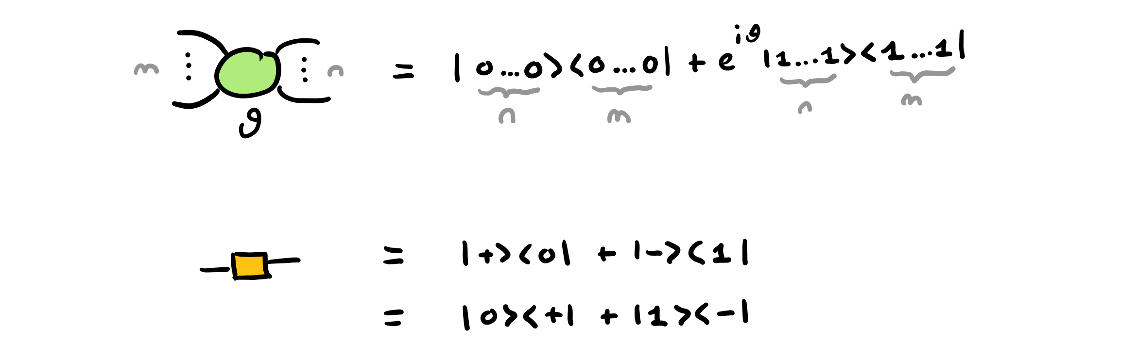
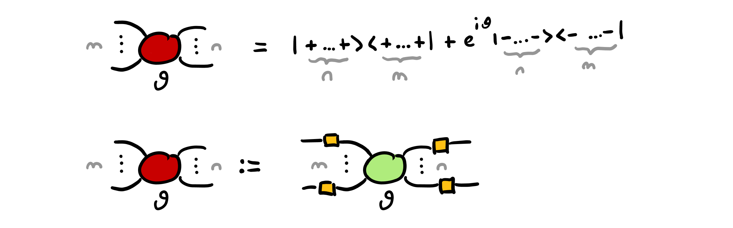
The X spiders can be defined in terms of Z spiders, using H boxes on all edges to “change colour” (i.e. change basis, in linear algebra terms). They are shown below, alognside the corresponding bra-ket notation:
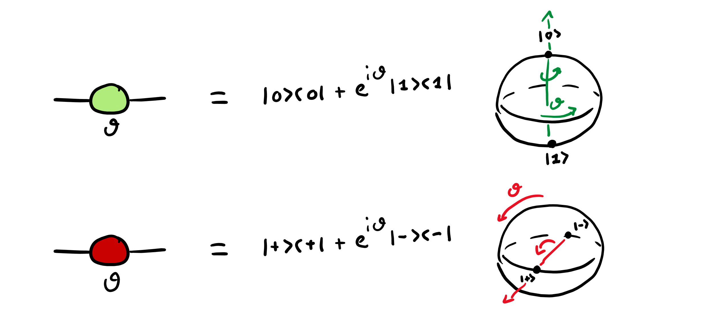
Spiders can be annotated by an angle, known as their “phase”; when omitted, the phase is set to 0 by convention. A spiders can have any number $m \geq 0$ of input legs and any number $n \geq 0$ of output legs, and it represents a linear map from $m$ qubits to $n$ qubits. We now discuss some special cases of immediate interest in quantum computing. The 1-to-1 spiders are single-qubit rotations, about the Z and X axis, respectively:
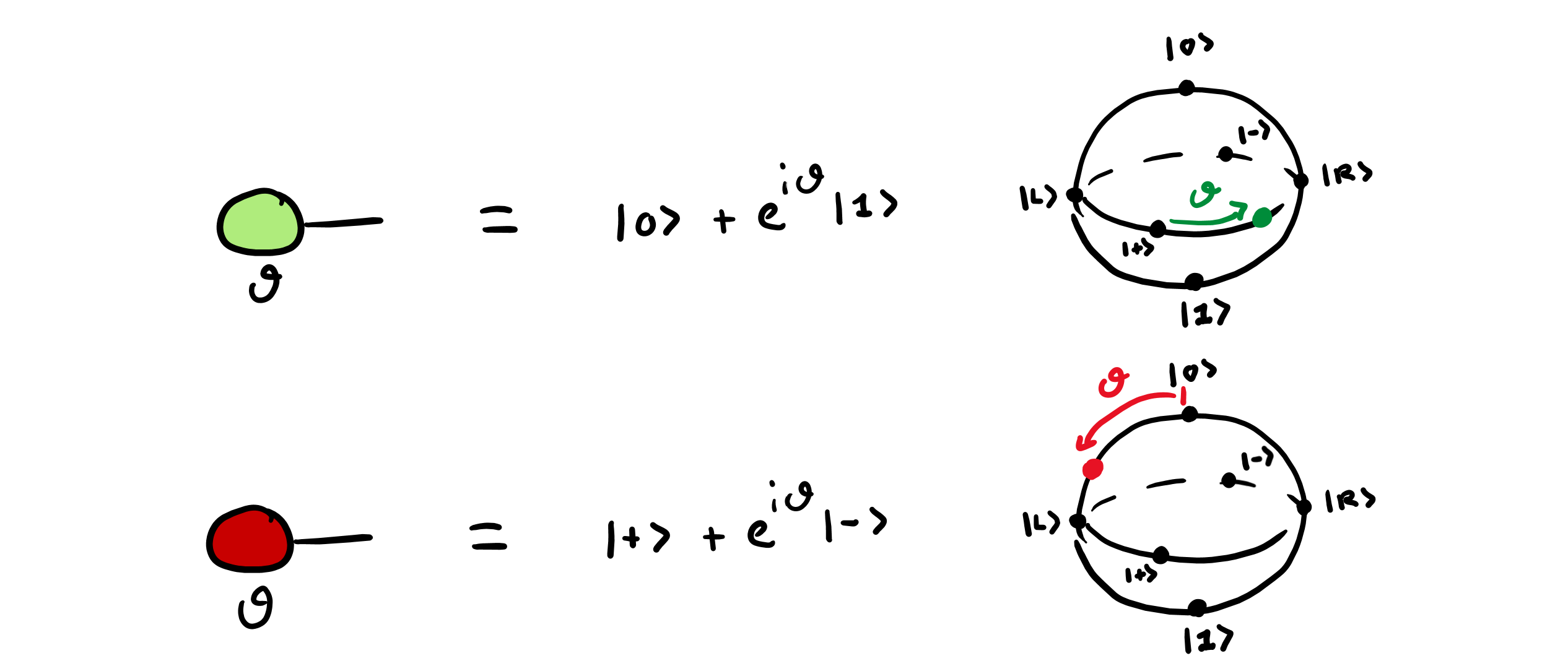
The 0-to-1 spiders represent the single-qubit states — column vectors, or “kets” — along the Z- and X-axis equator of the Bloch sphere, respectively:
The 1-to-0 spiders are the “adjoints” the states above — row vectors, or “bras” —:

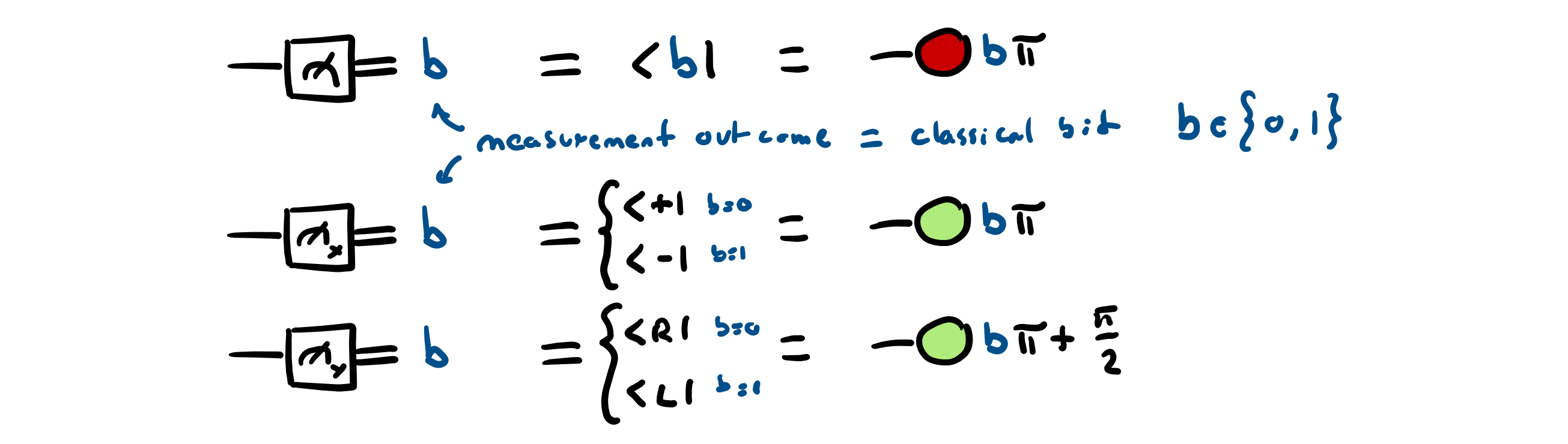
Specifically, some of these 1-to-0 spiders are used to represent the outcomes for measurements in the Z basis (the default measurement in digital quantum computing), the X basis, the Y basis, and certain other bases used in measurement-based quantum computing (not shown here):
Above, we have chosen the Z spiders and H boxes as the “generators” for the ZX calculus, its primitive building blocks, and defined the X spiders in terms of those generators. Alternatively, we could have taken Z spiders and X spiders as generators, and defined the H boxes in their terms, as follows:

The equation above is known as the Euler decomposition for the Hadamard gate, and it is a rewrite rule in our formulation of the ZX calculus. Alternatively, this equation could be taken to be the definition of the H box, and the defining equation of the X spiders would become a rewrite rule (known as the “colour change rule”).
For the ZX calculus to be useful in digital quantum computing, it has to be able to represent all possible fragments of quantum computation involving qubits. To show that the calculus possesses this property, known as “universality”, it is enough (cf. Section 4.5 of Nielsen and Chuang) to show that we can represent (i) all single-qubit rotations and (ii) the 2-qubit CNOT gate. By Euler decomposition for the Hadamard gate, all single-qubit rotations can be obtained as a sequence of three alternating Z-X-Z rotations, for suitable choice of angles: we already introduced the necessary Z and X rotations above, as 1-to-1 spiders. For the CNOT gate, on the other hand, we need two new instances of spiders: the 1-to-2 “copy spider” and the 2-to-1 “XOR spider”, shown below:
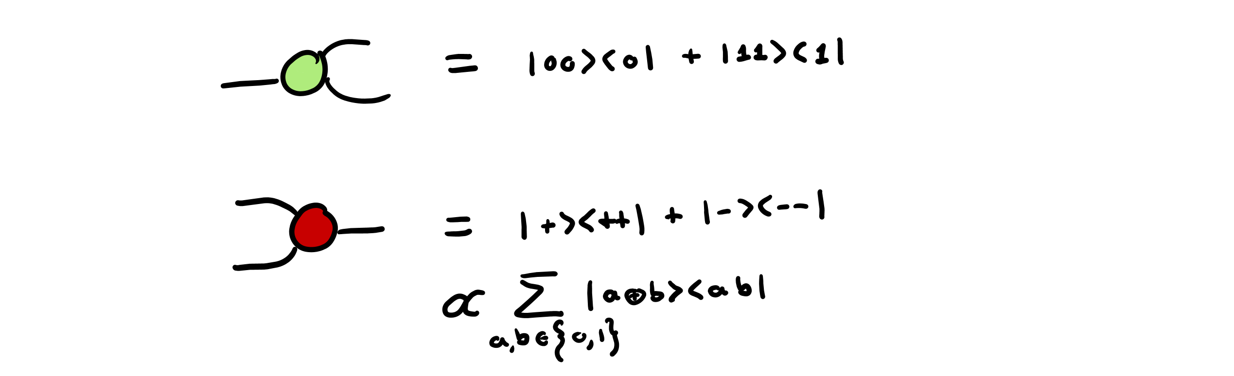
The copy spider produces copies of the Z basis states $\require{braket} \ket{0}$ and $\ket{1}$, while the XOR spider performs the XOR operation on the same basis, sending the 2-qubit Z basis state $\ket{a},\ket{b}$ to the 1-qubit Z basis state $\ket{a \oplus b}$. Combined, the copy and XOR spiders form the CNOT gate, the most common 2-qubit gate used in digital quantum computing: –>
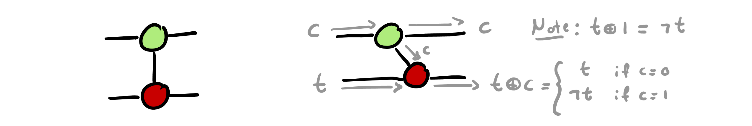
The definition of the CNOT gate above is perhaps the smallest useful example of a diagram, representing a quantum gate which is neither a rotation (represented by the Z and X 1-to-1 spider) nor the Hadamard gate (represented by the H box).
Diagrams vs Tensor Networks
ZX diagrams are undirected networks, with the exception of the dangling/open edges — known as “open legs” — which denote the input and output qubits of the quantum computation fragment. By convention, we read our diagrams left-to-right: open legs on the left are inputs, open legs on the right are outputs.
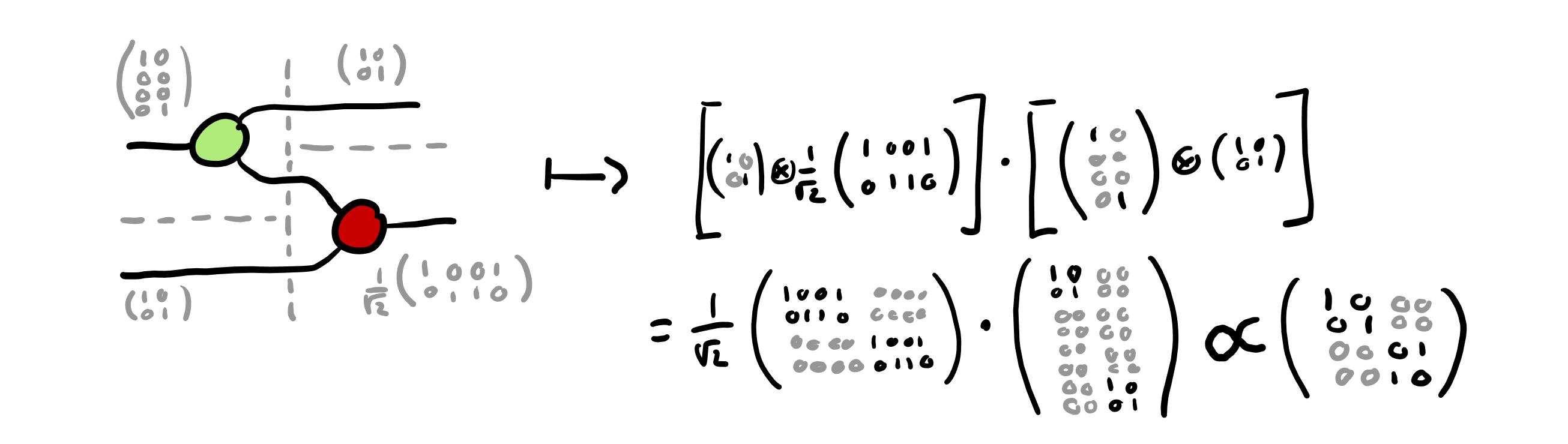
ZX diagrams with $m$ input legs and $m$ output legs represent $2^n$-by-$2^m$ complex matrices, which are composed in sequence by matrix multiplication and in parallel by Kronecker product. The example of the CNOT gate is shown below:
An equivalent — but significantly more flexible — semantics for ZX diagrams is as tensors in a tensor network, where each connection between spiders corresponds to a tensor contraction operation. The same example of a CNOT gate is shown below, using the Kronecker delta symbol $\delta_{x,y}$:
We will adopt the interpretation of spiders as tensors, rather than complex matrices, to exploit the additional flexibility of graph-theoretic contraction semantics for tensor networks over the parallel-and-sequential composition semantics of complex matrices. We will reserve “ZX diagram” to denote the abstract diagram itself, as a network of spiders and H boxes and use “tensor network” to denote the concrete numerical interpretation of a ZX diagram in terms of tensors to be contracted. For more on tensor networks and their efficient contraction, we recommend work by Gray and Kourtis, implemented in the cotengra library, and work on the Jet library by researchers at Xanadu.
Rewrite Rules
We have just seen that the ZX calculus is “universal”: it can represent all fragments of digital quantum computations. This makes it useful to write down quantum circuits, but not yet to reason about them. To gain reasoning powers, we need to introduce “rewrite rules”: these are equations relating pairs of diagrams which correspond to the same concrete fragment of computation, i.e. ones whose corresponding tensor networks contract to the same overall tensor. There are several broadly equivalent presentations for the rules of the ZX calculus: here, we will follow the presentations from Section 3.2 of Miriam Backens’s PhD Thesis and Section 2.2 of Harny Wang’s PhD Thesis.
An important fact about rewrite rules for the ZX calculus is that they come in pairs, related by “colour symmetry”. Given one rewrite rule, we can obtain another rule by swapping colours everywhere: every Z spider (green/light) in the original rule becomes an X spider (red/dark) in the new rule, and vice versa every X spider in the original rule becomes a Z spider in the new rule. For sake of simplicity, we state only one version of each rule below. We have already seen the “Euler” rule, expressing the H box in terms of Z and X spiders:
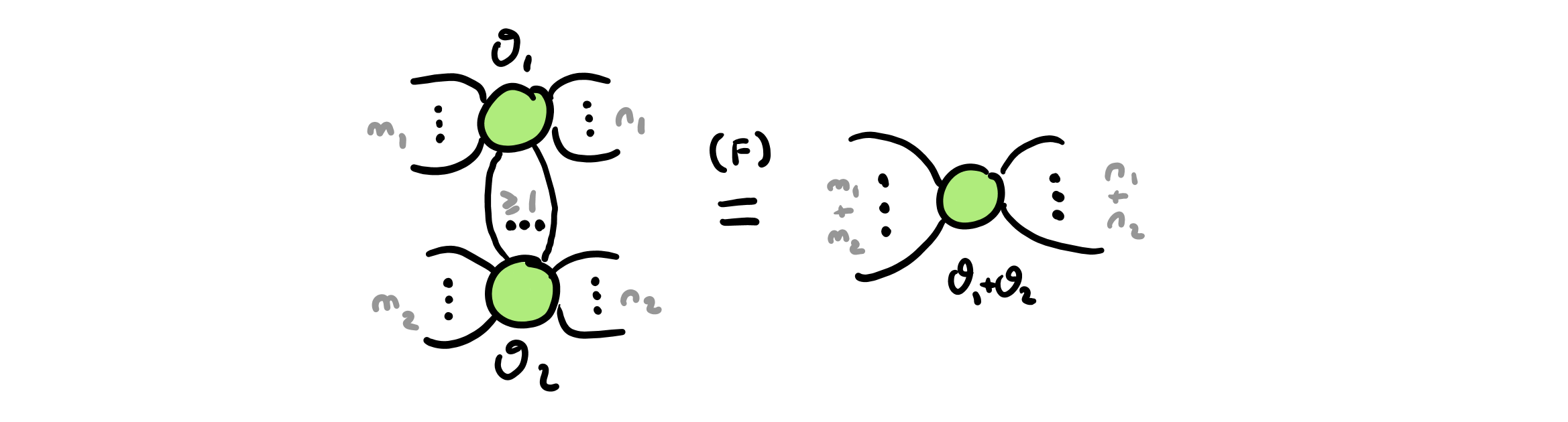
The “fusion rule” states that two spiders of the same colour connected by at least one leg can be fused into a single spider, adding the angles and preserving all legs connecting the original spiders to other parts of the diagram. Below we show the fusion rule for Z spiders:
The “identity rule” states that a spider with two legs and no phase can be removed, leaving an edge in its place. The “H squared” rule states that two H boxes connected can be removed, leaving an edge in their place. The identity rule for Z spiders and the H squared rule are shown below:

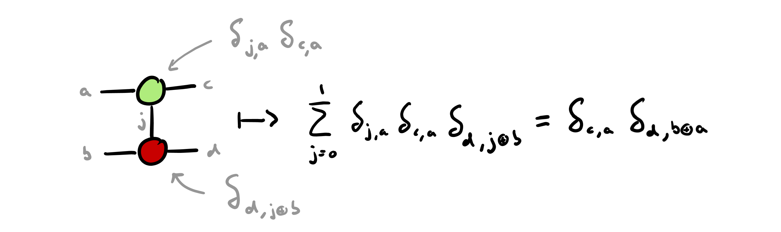
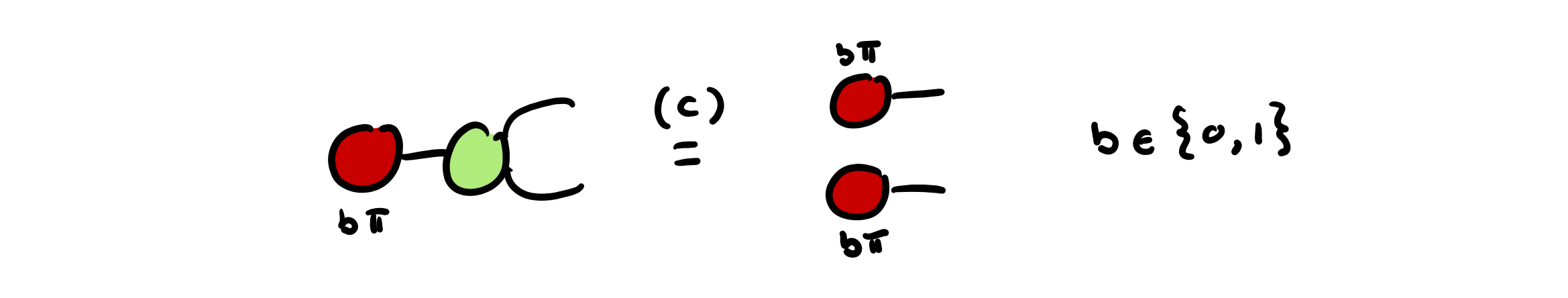
The “copy” rule states that the spider states with angle $0$ and $\pi$ of one colour are copied by the copy spider of the other colour. The copy rule for Z spiders, copying the Z basis states $\ket{0}$ and $\ket{1}$ — the X spider states with phases $0$ and $\pi$, respectively — is shown below:
The “$\pi$ commutation” rule states that an $\pi$ rotation in one colour can be commuted through a spider of the other colour, by being copied/broadcast to all other legs and negating the spider angle. The rule to commute X rotations by $\pi$ through Z spiders is shown below:

The “bialgebra” rule allows us to interchange …

A consequence of the bialgebra, copy and fusion rules is the “Hopf” rule. Shown below, the Hopf rule states that edges between spiders of different colours can be removed in pairs:

The fusion and Hopf rules and it can be used to reduce ZX diagrams from undirected multigraphs to undirected graphs, by fusing all connected spiders of the same colour and reducing the number of legs between spiders of different colour to either 0 or 1. The resulting diagrams are known as graph-like ZX diagrams, and play an important role in quantum circuit optimisation.
Where do we go from here?
As we stressed in the beginning, ZX calculus is a very important component of our technical toolkit. In the next posts, we will often piggyback to this page to show how it is used. Stay tuned!