
Part of the 20[ ] team has been busy in the last week with a research retreat focused on obstructions to compositionality. In this post, I’ll explain how this may have a direct role in better understanding intent search.
Recap and Introduction
If you recall, a few months ago we gave a Lagrangian account of what intent solving was. To recap:
- We have a graph where:
- Vertices are (EVM) states;
- Edges represent actions that lead from a state to another (e.g. calling a function with a given payload);
- An intent specifies a couple of regions in this graph:
- One region indentifies the premises of the intent, that is, the states in which intent search can be triggered;
- The other region identifies the conclusions of the intent, that is, the states that the intent proposer considers as acceptable solutions;
- Solving the intent means finding a path connecting these regions;
- The intent solver wants to find the path that best maximizes its revenue, or any other utility function (e.g. welfare).
This is a hard problem, and we’d really like it to be compositional. Compositionality is a pervasive idea in engineering. In a very handwavy way, we can say that:
Compositionality is the study of why and how properties of a given system can be inferred from the properties of its parts. Dually, it is the study of how to lift properties of smaller systems to the property of the system obtained by composing them according to some rule.
Breaking this down, we usually build complex systems by first building some pieces in isolation and then gluing them together. This is very well known to developers that first implement modules and libraries and then tie everything together into a final product. Such approach is called modular - or, in crypto circles, composable - and I have written about how this is different from compositionality some time ago. In a nutshell, Compositionality is stronger than modularity or composability: Modularity means being able to compose things, whereas compositionality means that some proprieties of the components (e.g. being ‘safe’ according to some spec) lift to the composed system (‘a system made by composing safe components is guaranteed to be safe’).
Simple examples of non-safe modular systems are:
- Plugs and sockets: You can stick a needle into a socket and get electrocuted. So the system is modular (the needle fits the socket) but non-compositional with respect to safety.
- Gas tanks: You can pour any fluid into a car’s gas tank using a funnel, which makes the system modular. Still, the composite system (fluid-into-funnel-into-car) is not necessarily compositional with respect to the car ever starting again.
Why should I care?
The reason why compositionality is relevant for us is that solving intents compositionally is a powerful thing:
Suppose you have an intent, expressed as the problem of finding the ‘best’ path to go from region $A$ to region $B$ of some graph, according to some definition of ‘best’. Ideally, we would like to:
- Finding some intermediate regions $I_0, \dots, I_n$;
- Finding the best paths from $A$ to $I_0$, from $I_0$ to $I_1$ and so on, all the way up to $I_n$, $B$;
- Having a way to glue these paths together, such that the resulting path is the best path from $A$ to $B$.
In the context of Lagrangian intents, this means that given an intent from the perspective of a solver $\mathfrak{s}$, that is, a triple $(T^\mathfrak{i,s} S, S^\mathfrak{i,s}_i, S^\mathfrak{i,s}_f)$, and given some Lagrangian $\mathcal{L}$ defining our concept of ‘best’, we would like to be able to split the search problem into subproblems, in such a way that finding paths that minimize the Lagrangian action $\mathcal{A}^\mathfrak{s}$ for the subproblems results in a path that minimizes $\mathcal{A}^\mathfrak{s}$ for the overall intent.
As you can see, having a compositional account of intent solving is a powerful concept, because:
- It gives us a hell of a computational advantage, since we know we can break a complicated intents into computationally simpler pieces and solve them separately;
- It gives an easy way to bundle intents, as we can solve single intents separately and then bundle the solutions together, while being reassured that no single intent gets solved suboptimally.
…But is this possible?
Compositionality is a very powerful property to have, and it is rarely satisfied in practice. That is, the class of problems that are truly compositional is rather small. I have been studying compositionality in abstract terms for the last 8 years, and recently, together with some colleagues, we’ve been increasingly focusing on characterizing reasons why compositionality fails for a given problem. We call these obstructions to compositionality. Hopefully, this sort of information will be useful to pinpoint subclasses of problems that exhibit less pathological behavior.
Understanding this in the context of intent solving could mean that whereas solving and bundling general intents is computationally a very hard problem, focusing on particular subclasses of intents - such as atomic swaps - will remove many computational hurdles, making the restricted problem tractable.
Even more practically, the formal study of obstructions to compositionality can be a useful tool to inform an intent solver about where are the low hanging fruits one can focus on.
Setting the stage
In this post, I’ll explain the approach to obstructions to compositionality that I have worked out with several coauthors in a homonimous paper. I redirect you there for a more formal treatment of this topic.
Open Graphs
To illustrate how our technique works, let’s consider the following example.
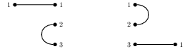
An open graph is a graph as below:

Intuitively, it is a graph with ‘open interfaces’, in this case the sets $\{1\}$ and $\{1,2,3\}$.
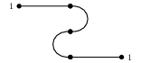
If we have two open graphs, and if their interfaces match:
Then they can be composed in the obvious way:
Now, suppose that we want to map each graph to the reachability relation between its interfaces. This means that, for instance, we want to map the open graph:
to a relation between the sets $\{1\}$ and $\{1,2,3\}$, where the only element in $\{1\}$ will be related to an element in $\{1,2,3\}$ if only if the corresponding open graph connects them. We see that in this case this relation is empty since there is no way to reach any point in the right interface if you start from the left interface.
As we can compose open graphs if their interfaces match, so we can compose relations:
Suppose that you have a relation $R$ between sets $A$ and $B$, and a relation $S$ between sets $B$ and $C$. One can define a composed relation $R;S$ between sets $A$ and $C$ by:
$a \in A$ is related to $c \in C$ through $R;S$ if and only if there exists $b \in B$ such that $a \in A$ is related to $b \in B$ through $R$ and $b \in B$ is related to $c \in C$ through $S$:
\((a,c) \in R;S \iff \exists b \in B. ((a,b) \in R \wedge (b,c) \in S).\)
So when we have two composable open graphs we can choose to either evaluate the reachability relations on the components and then compose the relations, or to compose the graphs first and then evaluate the reachability on the composition. Ideally, we would like these two operations to coincide: If calculating the reachability relation scales badly with respect to the size of the graph, we could take a computational shortcut by calculating the relation on the components and then gluing them together, and be guaranteed of not missing any possible solution.
Alas, this is not the case. To see why, let’s look again at the picture in Example 2: Call the graph on the top left $G$ and the graph on the top right $H$. The graph at the bottom is their composition, $G;H$. If we map each graph to the reachability relation on it, then $G$ goes to the relation $\{1\} \xrightarrow{\mathfrak{R}G} \{1,2,3\}$, which as we already remarked is emtpy. Similarly, $H$ goes to the empty relation $\{1,2,3\} \xrightarrow{\mathfrak{R}H} \{1\}$. These two can be composed into a relation $\{1\} \xrightarrow{\mathfrak{R}G;\mathfrak{R}H} \{1\}$, which applying relation composition is again empty. …On the other hand, if we evaluate the relation on the composite $\{1\} \xrightarrow{G;H} \{1\}$, this amounts to compute the reachability relation between the interfaces connected by the graph $G;H$. This relation is not empty at all, as we can clearly go from the $1$ on the left to the $1$ on the right!
So, we have $\mathfrak{R}G;\mathfrak{R}G \subseteq \mathfrak{R}(G;H)$, and the intuitive reason for this is that in composing $G;H$ we created a ‘zig-zag path’ that wasn’t there before.
With this, we established that the reachability problem for open graphs is non-compositional: evaluating reachability on the components misses out some solutions (in this case all of them) on the composite. Moreover, we also established that there is a function $\mathfrak{R}G;\mathfrak{R}G \subseteq \mathfrak{R}(G;H)$ - in this case even more than a function, an inclusion - and that compositionality fails precisely because this function is not invertible - that is, it is not a bijection.
This example is not an outlier: Indeed, almost all compositional problems can be rephrased in a similar way. Formally:
- We organize our problem and solution domains (in the case above open graphs and relations) into mathematical structures called categories;
- We encode our problem into a mapping between these categories (as we mapped open graphs to their reachability relations above);
- This mapping will be almost invariably a lax or an oplax functor;
- Our problem will be compositional precisely when this (op-)lax functor is strong;
- Characterizing obstructions to compositionality means characterizing obstructions for this functor to be strong.
There are a lot of definitions in the list above - category,functor- that would require a lot of time to unpack, but this is not important at the moment: What is important is understanding that a lax functor is strong precisely when a particular ‘function’ (more precisely a morphism in some category of functors and natural transfomations between them) is invertible.
So, as we can characterize obstructions to compositionality in the open graph problem by studying obstructions to some function being invertible, so we can study obstructions to compositionality for any problem by studying if some morphism (that is, a fancier generalization of function) is invertible. All this is to say that what we are doing in this toy example directly generalizes to much more complicated classes of problems.
From invertibility to terminality
In the following, I will use the word morphism quite a lot. morphisms are just a generalization of the concept of function. Functions are defined between sets - e.g. $A \xrightarrow{f} B$ is a function from set $A$ to set $B$. More generally, morphisms are defined between objects in some environment called a category. If this confuses you, in the reminder of this post you can think ‘function’ or ‘path’ or ‘a transformation of sorts’ almost every time you read ‘morphism’.
Ok, so our new problem at hand is: Given a morphism $f: A \to B$, when is it invertible? First of all, a formal definition:
A morphism $f: A \to B$ in a category $\mathcal{C}$ is called invertible, or equivalently an isomorphism, if there is another morphism $f^{-1}: B \to A$ such that:
\(\begin{align*} A \xrightarrow{f} B \xrightarrow{f^{-1}} A &= A \xrightarrow{id_A} A\\ B \xrightarrow{f^{-1}} A \xrightarrow{f} B &= B \xrightarrow{id_B} B \end{align*}\)
We see that this definition of invertibility, in the case of functions, coincides precisely with what we expect: A function is invertible precisely when it is bijective - here $id_A$ is just the function that sends any element of $A$ to itself, whereas $A \xrightarrow{f} B \xrightarrow{f^{-1}} A$, also denoted $f;f^{-1}$, is just function composition (apply $f$, then apply $f^{-1}$).
If $f:A \to B$ is invertible, then for any other morphism $g:X \to B$ there is exactly one morphism $h: X \to A$ for which we have $g = h;f$, or, as we category theorists like to say, for which this diagram commutes:
To see that $h$ exists it is enough to set $h = g;f^{-1}$:
Again, in the case of functions, consecutive arrows just denote function composition. “The diagram commutes” means “paths that start and end in the same endpoints are equal”, so from the diagram above:
\[\begin{align*} h;f &= (g;f^{-1});f\\ &= g;(f^{-1};f)\\ &= g;id_B\\ &= g. \end{align*}\]With this intuition in mind, interpreting these diagrams should be easy.
To see that $h$ is unique, suppose that there are two morphisms that make the triangle commute:
If $f$ is invertible, then:
\[\begin{align*} h_0 &= h_0;id_A\\ &= h_0;(f;f^{-1})\\ &= (h_0;f);f^{-1}\\ &= (g;f);f^{-1}\\ &= (h_1;f);f^{-1}\\ &= h_1;(f;f^{-1})\\ &= h_1;id_A\\ &= h_1\\ \end{align*}\]In jargon, we say that $g$ factors through $f$ uniquely. So, we have:
A morphism $f:A \to B$ is invertible if and only if any other morphism $g:X \to B$ factors through it uniquely.
This proposition is an if and only if, so if $f$ is not invertible there will always be some $g: X \to B$ that does not factor through it. Hence, such a $g$ can be seen as an obstruction to $f$’s invertibility.
There are two ways in which such a $g$ can fail to factor uniquely through $f$:
- Obstructions of the zeroth kind: $g$ doesn’t factor through $f$ at all, that is, there is no $h$ that makes the triangle commute:
- Obstructions of the first kind: $g$ factors through $f$ in multiple ways, that is, there are at least two $h_0 \neq h_1$ for which the triangle commutes:
Now, the conceptually hard part. If you squint your eyes enough, you’ll notice that the morphism $h$ in Figure 1 is somehow a ‘morphism between morphisms’: What I mean is that, through $h$, we can map $g$ into $f$. So yes, $h$ goes from $X$ to $A$, but changing perspective, we could also write:
\[h: g \to f.\]Embracing this, we can depict morphisms to a fixed object $B$ (such as $f$ and $g$) as points of some space (or object of a category, for the mathematically aware), and morphisms that make the triangles as the one in Figure 1 commute as directed paths (morphisms) in this space.
Having taken this conceptual leap, saying that $f:A \to B$ is invertible amounts to say that for any other point in this space, there is exactly one directed path to $f$. For the mathematically versed, this is made formal by saying that:
A morphism $f:A \to B$ in a category $\mathcal{C}$ is invertible if and only if it is a terminal object in the slice category $\mathcal{C}/B$.
So we transformed our problem once more. Instead of studying obstructions to invertibility directly, we resolved to study obstructions to terminality, that is:
A point in some space (e.g. a topological space, or a graph) is terminal precisely when, for any other point, there is exactly one directed path to it.
…Can we qualitatively describe obstructions for a point to have this propriety?
In a way that mimicks verbatim our considerations regarding invertible morphsims, a point - call it $\mathtt{1}$ - fails to be terminal precisely when one of the following two conditions is satisfied:
Given a space $\mathcal{C}$ and a chosen point $\mathtt{1}$, an obstruction of the zeroth kind for $\mathtt{1}$ in $\mathcal{C}$ is a point $x$ from which $\mathtt{1}$ is not reachable:
Given a space $\mathcal{C}$ and a chosen point $\mathtt{1}$, an obstruction of the first kind for $\mathtt{1}$ in $\mathcal{C}$ is a point $x$ from which $\mathtt{1}$ is reachable through different directed paths:
The zeroth homotopy poset
For now, we resolve to qualify obstructions of the zeroth kind for a chosen point $\mathtt{1}$ in some directed space (or more precisely, in some category) $\mathcal{C}$. The idea is to build a poset capturing qualitative information about the obstructions in question.
Posets
A poset is a set $P$ with a relation $\leq$ on it that is:
- Reflexive: for every element $p$ of $P$, it is $p \leq p$;
- Antisymmetric: For all $p,q \in P$, if $p \leq q$ and $q \leq p$, then $p=q$;
- Transitive: For all $p,q,s \in P$, if $p \leq q$ and $q \leq s$, then $p\leq s$.
The most obvious example of posets are the integers, with the usual ‘less or equal’ relation on them. This is a boring poset since for any couple of numbers $n,m$, either $n \leq m$, $n = m$ or $n \geq m$. A more interesting example is, say, $n \times n$ matrices over the integers. In this case we can set $M \leq N$ if for every $0 \leq i,j \leq (n-1)$, the $ij$-th entry of $M$ is less or equal than the $ij$-th entry of $N$. It is easy to see that the $\leq$ so defined respects the Poset axioms, and so the set of all $n \times n$ integer matrices is a poset under this relation. In this poset not all elements are comparable: For instance, considering the matrices
\[\mathbf{0} = \left(\begin{matrix}0 & 0\\ 0 & 0\end{matrix}\right) \qquad M = \left(\begin{matrix}1 & 0\\ 1 & 0\end{matrix}\right) \qquad N = \left(\begin{matrix}0 & 1\\ 0 & 1\end{matrix}\right)\]we see that $\mathbf{0} \leq M$, $\mathbf{0} \leq N$, but $M$ and $N$ are not comparable: $M \not\leq N$, $N \not\leq N$.
Defining the zeroth homotopy poset
Now we build a poset out of our starting space by squeezing out redundant information:
Given two points $x, y$ in $\mathcal{C}$, we set $x \leq y$ if there is a directed path from $x$ to $y$. The resulting poset is called the poset reflection of $\mathcal{C}$.
If we have directed paths $x \to y$ and $y \to x$, then $x \leq y$ and $y \leq x$, and because of the antisymmetric property of $\leq$, $x = y$. Hence, we are contracting points among which we can freely move. Similarly, it doesn’t matter how many directed paths there are between $x$ and $y$, as long as there is at least one, we will have $x \leq y$. Hence, we are intentionally forgetting about multiple ways to go from $x$ to $y$ (remember we’re focusing on obstructions of the zeroth kind).
Now, we make a further step: We do not care about any point $x$ such that $x \leq \mathtt{1}$ as by definition this means that there is at least directed path from $x$ to $\mathtt{1}$, and so $x$ cannot be an obstruction of the zeroth kind. So, we identify all of these ‘trivial’ points, and we write $[\mathtt{1}]$ for the ‘generalized point’ including any $x$ as above. Notice that $[\mathtt{1}]$ also includes $\mathtt{1}$ since obviously $\mathtt{1} \leq \mathtt{1}$.
For the mathematically versed, we are quotienting the poset by the downset generated by $\mathtt{1}$.
Given some space $\mathcal{C}$ and a chosen point $\mathtt{1}$, the poset hereby defined is called the zeroth homotopy poset associated to $\mathtt{1}$, and is denoted $\pi_0\left(\mathcal{C}/\mathtt{1}\right)$.
If you know a bit of topology, you should notice that the nomenclature ‘homotopy poset’ is not casual: If $G$ is a groupoid, then $\pi_0\left(G/\mathtt{1}\right)$ is a set, that is, a discrete poset. Regarded as a set pointed in $\mathtt{1}$, it is isomorphic to the set $\pi_0(G)$ of the connected components of $G$, pointed at the conected component associated to $\mathtt{1}$. Our $\pi_0$ is nothing more than a ‘directed generalization’ of the $\pi_0$ from homotopy theory.
Structure of $\pi_0\left(\mathcal{C}/\mathtt{1}\right)$
It makes sense to highlight some basic facts about the structure of $\pi_0\left(\mathcal{C}/\mathtt{1}\right)$:
For any given $\mathcal{C}$ and chosen point $\mathtt{1}$, the structure of $\pi_0\left(\mathcal{C}/\mathtt{1}\right)$ is as follows:
- Trivially, $[\mathtt{1}] \leq [\mathtt{1}]$.
- If $y \neq [\mathtt{1}]$, it is never the case that $y \leq [\mathtt{1}]$. Indeed, $y \leq [\mathtt{1}]$ means $y \leq x$ for some $x \in [\mathtt{1}]$, which by definition means $x \leq \mathtt{1}$. So $y \leq x \leq \mathtt{1}$ and, by transitivity, $y \leq \mathtt{1}$. Hence, by construction, $y$ is in $[\mathtt{1}]$ as well: Such a point $y$ doesn’t really exist anymore in our poset, it has been absorbed by $[\mathtt{1}]$.
- If there is $x \in [\mathtt{1}]$ such that $x \leq y$, then $[\mathtt{1}] \leq y$. To visualize this, depict the premise graphically as follows:
Here the relation $\leq$ is depicted by putting the greater point above the lesser one. As we identify $x$ with $\mathtt{1}$ by construction, the whole left branch of this depiction collapses to a point, leaving us with the conclusion.
- For $x,y \neq [\mathtt{1}]$, $x \leq y$ if there is at least one directed path from $x$ to $y$.
In layman terms, our $\pi_0\left(\mathcal{C}/\mathtt{1}\right)$ ranks obstructions of the zeroth kind ‘by size’: If we removed an obstruction $y$ by adding a directed path $y \to \mathtt{1}$, then we’d automatically remove also all obstructions $x \leq y$, since these too could now reach $\mathtt{1}$ by passing through $y$. $[\mathtt{1}]$, a point representing ‘non obstructions’, is ranked lowest in the poset structure.
Calculating a simple $\pi_0$
As an example, let’s calculate the zeroth homotopy poset for the function $f: \{0,1\} \to \{0,1,2,3\}$ that maps $0 \mapsto 0$ and $1 \mapsto 1$. Our $\pi_0$ will classify functions $X \to \{0,1,2,3\}$ for which there is no $h: X \to \{0,1\}$ which makes the following triangle commute:
- At the bottom of our $\pi_0$ there is $[f]$, a point representing the image of $f$ in $B$, which is again $\{0,1\}$. Indeed, any $g$ that hits only $0$ or $1$ in $\{0,1,2,3\}$ can factor through $f$, so it’s not an obstruction. This is the only minimal element of the poset.
- Right above $[f]$ we have two points, which overloading notation we define as $\{2\}$ and $\{3\}$. These represent two functions $\{*\} \to \{0,1,2,3\}$ only picking $2$ and $3$, respectively. It is easy to see that for these functions there is no way to close the commutative triangle, since $f$ never hits $2$ or $3$. Moreover the following triangles commute:
So the empty function is $\leq$ than both $f$ and $\{2\}$, and according to our characterization of the zeroth homotopy poset, $[f] \leq \{2\}$. A similar argument holds for $\{3\}$.
- Above $\{2\}$ and $\{3\}$ there are functions that hit either $2$ or $3$, and exactly one other element between $0$ and $1$.
- Above those, there are functions that hit any three elements in $\{0,1,2,3\}$.
- At the top of the poset, there is the identity function on $\{0,1,2,3\}$.
Any other function from any set $X$ to $\{0,1,2,3\}$ can be shown to be equal to one of the elements in this poset. Consider for instance the function $g: \{a,b\} \to \{0,1,2,3\}$ that maps both $a,b$ to $2$. $g$ factors through the function $\{2\} : \{*\} \to \{0,1,2,3\}$ by sending both $a,b$ to $*$. Similarly, the function $\{2\}$ factors through $g$ by sending $*$ either to $a$ or to $b$. So $g \leq \{2\}$ and $\{2\} \leq g$, and hence $g = \{2\}$. All in all, all the obstructions of the zeroth kind for $f$ are classified by the following poset:
This means that in the case of functions between sets, obstructions of the zeroth kind are precisely obstructions to surjectivity. Furthermore, any surjective function will have a trivial $\pi_0$ consisting of only one element, meaning that ‘nothing is an obstruction’.
The first homotopy poset
Now, we want to capture obstructions of the first kind, that is, points from which our chosen element $\mathtt{1}$ is reachable through different directed paths. We want to do as little work as possible, and indeed, we will show how the first homotopy poset is nothing more than the zeroth homotopy poset calculated in some other space.
Defining the first homotopy poset
Again, let us fix some space $\mathcal{C}$ and a point $\mathtt{1}$. An obstruction of the first kind is a point $x$ that reaches $\mathtt{1}$ in at least two different ways:
Now, consider this weirdly-shaped diagram:
If both triangles commute at the same time, then it is:
\[\begin{gather*} h_0 = h ; id_\mathtt{1} = h\\ h_1 = h ; id_\mathtt{1} = h \end{gather*}\]And so $h_0 = h_1$. This is clearly an if and only if: There is no way to make both triangles commute at the same time if $h_0$ and $h_1$ are different.
To understand where this triangle ‘lives’, consider a new space where points are couple of paths $x \xrightarrow{f_0,f_1} \mathtt{1}$, and where a - higher level, if you wish - path from point $x \xrightarrow{f_0,f_1} \mathtt{1}$ to point $y \xrightarrow{g_0,g_1} \mathtt{1}$ is a path $x \xrightarrow{h} y$ which makes both these triangles commute:
Given a space $\mathcal{C}$ and a chosen point $\mathtt{1}$, we call the space we just constructed $\text{Par}\left(\mathcal{C}/\mathtt{1}\right)$.
With this intuition, we see that we reconducted obstructions of the first kind to $1$ in $\mathcal{C}$ to obstructions of the zeroth kind to $\mathtt{1} \xrightarrow{id_\mathtt{1},id_\mathtt{1}} \mathtt{1}$ in $\text{Par}\left(\mathcal{C}/\mathtt{1}\right)$. But these we already know how to classify!
Given a space $\mathcal{C}$ and a chosen element $\mathtt{1}$, the first homotopy poset associated to $\mathtt{1}$, denoted $\pi_1\left(\mathcal{C}/\mathtt{1}\right)$, is defined as:
\[\pi_1\left(\mathcal{C}/\mathtt{1}\right) = \pi_0\left(\left(\text{Par}\left(\mathcal{C}/\mathtt{1}\right)\right)/(id_\mathtt{1},id_\mathtt{1})\right).\]Again, if you know topology, you may notice that if $G$ is a groupoid, then $\pi_1\left(G/\mathtt{1}\right)$ is again a set, that is, a discrete poset. Regarded as a pointed set, it is isomorphic to the underlying pointed set of the group $\pi_1(G, \mathtt{1})$ of the loops at $\mathtt{1}$. Indeed, the definition
\[\pi_1\left(\mathcal{C}/\mathtt{1}\right) = \pi_0\left(\left(\text{Par}\left(\mathcal{C}/\mathtt{1}\right)\right)/(id_\mathtt{1},id_\mathtt{1})\right)\]Mimicks what happens in topology, where denoting as $\Omega(X,x)$ the space of loops in a space $X$ pointed at $x$, and as $c_x$ the constant path at $x$, we define:
\[\pi_1\left(X,x\right) = \pi_0\left(\Omega \left(X,x\right),c_x\right).\]Hence, you can view $\text{Par}\left(\mathcal{C}/\mathtt{1}\right)$ as a directed version of the loop space.
Calculating a simple $\pi_1$
A characterization of $\pi_1\left(\mathcal{C}/\mathtt{1}\right)$ can be obtained applying the characterization of the zeroth homotopy poset to the definition of $\pi_1\left(\mathcal{C}/\mathtt{1}\right)$. That’s a lot of piggybacking, and it’s not worth to cover in this post. Instead, it is probably more useful to compute $\pi_1$ for a simple function.
Let $f:\{0,1\} \to \{*\}$ the function that sends both $0,1$ to $*$, and let us calculate its $\pi_1$. This poset will classify functions $g : X \to \{*\}$ for which there are two different functions $h_0, h_1$ that make the following triangle commute:
Remember that our $\pi_1$ is defined in terms of $\pi_0$ on the space of parallel paths. Hence, if $g$ is an obstruction of the first kind for $f$, then the couple of paths $(h_0,h_1)$ is an obstruction of the zeroth kind to $(id_f,id_f)$. Keeping track of all this bookkeeping can be complicated, but we can try to visualize everything with a diagram like the one below:
In this diagram we depict functions in blue, functions seen as ‘paths between functions’ in black, and functions seen as ‘paths between paths between functions’ in red, so that we can try to keep track of how things act at different levels. The diagram says that $g$ is an obstruction of the first kind for $f$ if and only if $h_0 \neq h_1$, if and only if $(h_0, h_1)$ can’t factor through $(id_{\{0,1\}},id_{\{0,1\}})$. This means that there is no path from the former to the latter, and so that $(h_0, h_1)$ is an obstruction of the zeroth kind for $(id_{\{0,1\}},id_{\{0,1\}})$.
As $\pi_1$ is defined in terms of $\pi_0$ on the space of parallel paths, in the poset $\pi_1$ every $g$ is classified in terms of the couples of parallel functions that go from $g$ to $f$. These will be couples of parallel functions from some set $X$ to $\{0,1\}$, the domain of $f$.
To keep the notation manageable, we will encode these pairs as sets of pairs made of $0$s and $1$s. The set itself represents the domain of the two functions. The first function is obtained by taking the first projection, the second function by taking the second. So, for instance, the set:
\[\\{(0,0),(0,1),(1,1)\\}\]Represents the following pair of functions $(h_0,h_1)$:
\[\require{extpfeil} \begin{align*} (0,0) \xmapsto{h_0} 0\\ (0,1) \xmapsto{h_0} 0\\ (1,1) \xmapsto{h_0} 1\\ (0,0) \xmapsto{h_1} 0\\ (0,1) \xmapsto{h_1} 1\\ (1,1) \xmapsto{h_1} 1 \end{align*}\]
Now, let’s finally describe our $\pi_1$.
- At the bottom of the poset, we find $[(id_{\{0,1\}},id_{\{0,1\}})]$ wich witnesses couples of equal arrows, that is, ‘non-obstructions’ of the first kind.
- Right above this, there is the couple $\{(0,1)\}$ (we are using our encoding here). Explicitly, this couple is given by the two functions $\{(0,1)\} \to \{0,1\}$ sending $(0,1)$ to $0$ and $1$, respectively. Since in our formalism pairs of functions do not commute, we also include $\{1,0\}$ as an independent element of the poset. To see why these elements are directly above $[(id_{\{0,1\}},id_{\{0,1\}})]$, consider $\{(0,1)\}$: following the rules of the zeroth homotopy poset, it will be
$\{(0,1)\} \leq [(id_{\{0,1\}},id_{\{0,1\}})]$ if we can find some other couple $(x,y)$ such that $(x,y) \leq (0,1)$ and $(x,y) \leq (id_{\{0,1\}},id_{\{0,1\}})$. The couple in question is a pair of empty functions, as can be seen in the following - terrible - diagram:
- One level above, we have the sets $\{(1,1),(0,1)\}$, $\{(0,0),(0,1)\}$, $\{(0,1),(1,0)\}$, $\{(1,1),(1,0)\}$ and $\{(0,0),(1,0)\}$. These are all pairs of functions from a two element set to $(0,1)$, that disagree on at least one value.
- One level above, we have $\{(0,0),(0,1),(1,1)\}$, $\{(0,1),(1,0),(1,1)\}$, $\{(0,0),(0,1),(1,0)\}$ and $\{(0,0),(1,0),(1,1)\}$. These are all pairs of functions from a three element set to $\{0,1\}$, again disagreeing on at least one value.
- Finally, the top of the poset is composed by just one pair of functions from a four element set to $\{0,1\}$, namely $\{(0,0),(0,1),(1,0),(1,1)\}$.
All in all, the poset looks like this:
As for $\pi_0$, any $g:X \to \{0,1\}$ that is an obstruction of the first kind to $f$ will exhibit a number of non equal paths $(h_0,h_1)$, each one to be equal to one of the elements in the poset above.
Finally, you may have noticed that for functions $\pi_1$ acts in a dual way with respect to $\pi_0$. Indeed, for functions between sets, $\pi_1$ witnesses obstructions to $f$ being injective.
Closing remarks
If you made it so far, you may be thinking “what the actual fuck? You promised me a post about intents and everything I’m seeing is a bunch of horrendous math!”, and you would basically be right. But the fact is this: The theory we so far developed, and that I have tried to exemplify by means of very simple examples, can be applied to a wide, wide range of problems, among which graph reachability, which is deeply related to intent search as you may already know from our previous Lagrangian account. Indeed, we spent the best part of the paper we published by characterizing how homotopy posets behave in various contexts - how they relate to each other, how do they transform when your problem domain changes, and so on and so forth. The hope is that these complicated techniques may give us insights about what exactly makes intent solving and bundling difficult, and how to circumvent these difficulties.
Another approach that we have been developing at the workshop I mentioned, and on which I’m very bullish, is based on a possibly even more abstract tool called sheaf cohomology. The reason why I’m so bullish about it is that, whereas we still don’t know which way is the best to compute homotopy posets efficiently, the sheaf approach spits out, pretty much by design, computational lower bounds on the complexity of the problem at hand. When we realized that we were looking at results such as “if the n-th cohomology group of your sheaf is trivial, then your problem can be solved in linear time” it literally blew my mind away.
So, you can expect another followup post talking about sheaf cohomology in the future. This won’t be anytime soon tho, since we have a working paper to be published first. Stay tuned!
If you want to know more, do not forget to check out our paper, Obstructions to Compositionality.